Fourier Transforms (FT)

Broadly, the fourier transform is a way of transforming some vectors or functions into other vectors or functions. The fourier transform has a broad range of applications and is central in many mathematical fields, so depending on who you ask, the fourier transform is likely to mean different things.

If you ask a mathematician what a fourier transform is they are likely to reply with some gibberish that sounds like “the fourier transform is a linear operator that acts on Hilbert spaces and groups that satisfies a variety of nice properties (such as invertibility) under various conditions.”

A physicist will say “the fourier transfrom lies at the core of many fundamental fields in physics such as quantum mechanics and fluid dynamics. What’s more, the fourier transform is a essential to the math behind statistical mechanics, and its use is ubiquitous in computational modelling of physical systems.”

A signal processing engineer, i.e. an engineer in any of these fields: music; computer vision; stock market prediction; some medical fields such as EEG/EMG/ECG analysis; power grid/energy distribution; and more—will tell you that the discrete fourier transform is one of the most fundamental tools used in digital sigial processing.

In this repository we explore some algorithms for computing the discrete fourier transform of vectors.

Discrete Fourier Transform (DFT)

Fourier transforms are one of the workhorses of physics, both computational and otherwise. On a computer, we in generaly carry out discrete Fourier transforms or DFTs, where we sum (rather than integrate) over a discrete set of function points, and evaluate the DFT at a discrete set of \(k\)’s. Because of this, the DFTs can differ in some subtle ways from analytic Fourier transforms.

The DFT of a vector is a linear transformation which can be represented by a matrix. If the vector in question is \(n\) dimensional, and it’s either real or complex, then the DFT matrix is a linear operator \(\mathbb{C}^n\to\mathbb{C}^n\) (or \(\mathbb{R}^n\to\mathbb{C}^n\)). It looks like this

\[\begin{bmatrix} 1 & 1 & 1 & 1 & \cdots & 1 \\ 1 & e^{-2\pi i/n} & e^{-4\pi i/n} & e^{-6\pi i/n} & \cdots & e^{-(n-1)2\pi i/n} \\ 1 & e^{-4\pi i/n} & e^{-8\pi i/n} & e^{-12\pi i/n} & \cdots & e^{-2(n - 1)2\pi i/n} \\ 1 & e^{-6\pi i/n} & e^{-12\pi i/n} & e^{-18\pi i/n} & \cdots & e^{-3(n - 1)2\pi i/n} \\ \vdots & \vdots & \vdots & \vdots & \vdots & \vdots \\ 1 & e^{-(n-1)2\pi i/n} & e^{-2(n-1)2\pi i/n} & e^{-3(n-1)2\pi i/n} & \cdots & e^{-(n-1)^2 2\pi i/n} \end{bmatrix}\]

The matrix can be written more succinctly like so

\[a_{j,k} = \exp(-j\cdot k\cdot 2\pi i/n)\qquad\text{DFT} = (a_{j,k})\]

It is symmetric, orthogonal, and unitary (up to a factor of \(1/\sqrt n\)) i.e. it’s inverse is just \(1/n\) times it’s hermitian conjugate.

Properties of the DFT

mostly stolen from Jon’s note for this section

Inverse DFT

The inverse DFT is it’s hermitian conjugate (up to a scaling factor of N).

\[F^\dagger F x[t] = \sum_k \exp(2\pi ikt’/N) \sum_t \exp(-2\pi ikt/N) x[t] = \sum_t x[t] \sum_k \exp(-2\pi ik(t-t’)/N) = \sum_t x[t]N\delta(t-t’) = N x[t]\]

Shifted DFT

If we know the DFT of a function, we also can work out the DFT of a shifted version of the function.

\[F{x[t-m]}(k) &= \sum_t’ x[t’]\exp(-2\pi ik(t’+m)) = \exp(-2\pi ikm/N) F{x[t]}(k)\]

In words, we apply a phase ramp with slope $\exp(-2\pi im/N)$ to the original Fourier transform.

Flipped DFT

If we know the DFT of a function, the DFT of the flipped version $f(-x)$ is:

\[X(k) = \sum_t x[-t]\exp(-2\pi ikt/N) = \sum_t x[t]\exp(2\pi ikt/N) (\sum_t x^\ast[t] \exp(-2\pi ikt/N))^\ast\]

Which is the conjugate of the DFT of the conjugate of $x[t]$. For the special (but common) case that $x[t]$ is real, the DFT of $x[-t]$ is the complex conjugate of the DFT of $x[t]$.

Order of the DFT matrix

Up to scaling factor $\sqrt N$

The DFT matrix is an order four unitary transformation. i.e. $F\circ F\circ F\circ F x[t] = x[t]$. To see this we apply it twice.

\[\frac{1}{N}\sum_s \exp(-2\pi iks/N) \sum_t \exp(-2\pi ist/N) x[t] = \frac{1}{N} \sum_t x[t]\sum_s \exp(-2\pi is(k+t)/N) = \sum_t x[t]\delta(k+t)/N = x[-k]\]

Applying the DFT twice to $x[t]$ flips it to $x[-t]$. Therefore, if we apply it four times we retrieve our original data. It follows that $F^3 = F^\dag = F^{-1}$.

Aliasing

What if we want to know that DFT of some larger frequency $X[k+mN]$ for integer $m$? Well, that is

\[\sum_t x[t]\exp(-2\pi i(k+mN)t/N) = \sum_t x[t]\exp(-2\pi ikt/N)\]

So $X[k+mN] = X[k]$. Similarly if we take the inverse DFT $F^\dag {x[t]}(k+mN) = F^\dag {x[t]}(k)$.

While we usually only think about a single period of the DFT, in practice they repeat infinitely and you would do well to keep that in mind. In particular, a jump from the right edge of our function to the left edge looks just like a jump in the middle of our function - one way to see this is to apply a phase ramp from the shifting theorem to move the edge of the domain into the middle.

Similarly, if we have high frequency components in our data, where $k>N$, the DFT of those components are indistinguishable from componants where $0\leq N$. This can be a huge problem when applying DFT to signal processing and usually one uses analog (not digital) filters to make sure that frequency componants outside of your nyquist zone of interest are gone before the digital system ever sees the signals.

A ‘nyquist zone’ is the width of the largest piece of bandwidth that can be fully described by your data given your sampleing rate. More on this below.

DFT of Real Functions

Applying the flip thoerem to $X(k)$, we have $X(-k)= (F x[t]^\ast)^\ast$. When x[t] is real, then this reduces to $X(-k)=X(k)^\ast$. However, from aliasing we know that $X(-k)=X(N-k)$, so for real data, we have $X(N-k)=X(k)^\ast$. i.e. the second half of the DFT is just the flip of the conjugate of the first half. This is such a common case that Fourier transform libraries universally support the transforms of real data, and only return the first half of the DFT. You would generally do well to keep this aliasing in mind, and think of the highest frequences in the DFT as the lowest negative frequencies.

Sampling/Nyquist Theorem

We now have enough bits in place to understand one of the most fundamental theorems in digital signal processing. If we have a signal with maximum frequency $\nu$, how fast do we have to measure that signal to capture all its information? Naively, you might think if you had a signal with frequnecy up to 1MHz, that you would have to measure the signal one million times per second. This isn’t right, because really the signal generally has components from -1MHz to 1MHz, for a total width of 2MHz. That means you had better sample 2 million times per second to capture all the information in the signal.

Discrete Convolution theorem

Cross-correlations

2-dimensional DFTs

n-dimensional DFTs

Fast Fourier Transform FFT

The FFT is a family of algorithms for computing the DFT of a vector. It is by far the most popular algorithm—so much so that many people use FFT and DFT interchangably.

Cooley-Tukey Algorithms

Cooley Tukey Algorithms for the FFT are the most important class of fast fourier transform algorithms.

Radix-2 DIT

Note: DIT stands for ‘Decimation In Time’.

The Radix-2 algorithm is the simplest Cooley-Tukey algorithm. It assumes that the input vector (or ‘signal’) has exactly \(2^r\) dimensions (\(r\) is a positive integer). The algorithm shuffles the vector’s componants around, then splits the vector into two halves and reccursively applies it’s self to each half of the vector, and then re-combines the output of each.

Let \(x\) be a \(n = 2^r\) dimensional vector with real or complex entries

\[x = \big[ x[0] , x[1] , x[2] , … , x[n-1] \big]\]

And let \(X\) be it’s fourier transform.

\[DFT\{x\}[k] = X[k] = \sum_{t=0}^{n-1} x[t] e^{-t \cdot k\cdot 2\pi i / n}\]

The key insight is to realize that this sum is itsself the sum of two smaller sums that are each DFTs of subvectors of \(x\).

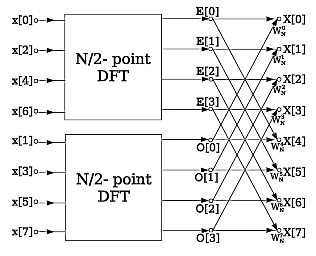
\[\sum_{t=0}^{n-1} x[t] e^{-t \cdot k\cdot 2\pi i / n} = \left( \sum_{t_0=0}^{n/2-1} x[2t_0] e^{-t_0\cdot k\cdot 2\pi i/(n/2)} \right) + e^{- k\cdot 2\pi i/n} \left( \sum_{t_1=0}^{n/2-1} x[2t_1+1] e^{-t_1\cdot k\cdot 2\pi i/(n/2)} \right)\] \[DFT\big\{ x[0] , x[1] , ... , x[n-1] \big\} = DFT\big\{ x[0] , x[2] , .. , x[n-2] \big\} \\ \hspace{15.0em} + e^{-k\cdot 2\pi i/n} DFT\big\{ x[1] , x[3] , ... , x[n-1] \big\}\]

Now you can see that the right hand side is just the sum of two smaller Fourier Transforms times a phase-ramp (formally known as twiddle factors). To solve those two, you reccursively apply the same trick until you get to two dimensional vectors where the Discrete Fourier Transform reduces to a trivial sum and difference.

\[DFT\{x[0] , x[1]\} = \big[ x[0] + x[1] , x[0] - x[1] \big]\]

Below: Butterfly diagram of the Culey Tukey FFT.

Python implementation

A recursive implementation

import numpy as np          # numpy library
PI = np.py                  # the constant 3.14...

def fft(arr):
  n = arr.shape[0]          # assume arr len is a power of 2
  if n == 1:
    return arr[0]
  else:
    even = fft(arr[::2])    # FFT of even indices
    odd = fft(arr[1::2])    # FFT of odd indices
    phase = np.exp(2*PI*1.j/n * np.arange(n/2))
    odd *= phase            # pointwise multiply odds by phase 
    return np.concatenate([even + odd , even - odd])

Radix 2 DIT in the Language of Linear Algebra

As you can see, the python implementation is very short and easy to read because python does most of the heavy lifting for us. In order to take a deeper dive and implement it at a lower level, it will be helpful to understand the Cooley Tukey algorithm as a matrix decomposition.

Using the formula that expresses a DFT in terms of two DFT’s of half the size that we derived just above, we will re-cast one DFT matrix as the product of three matrices. We will use \(n=8\) as a small but non-trivial example. To decompose our matrix, we notice that the first operation is to separate even indexed elements from the odd ones, so our right-most matrix will do just that:

\[S_8 := \begin{bmatrix} 1 & 0 & 0 & 0 & 0 & 0 & 0 & 0 \\ 0 & 0 & 1 & 0 & 0 & 0 & 0 & 0 \\ 0 & 0 & 0 & 0 & 1 & 0 & 0 & 0 \\ 0 & 0 & 0 & 0 & 0 & 0 & 1 & 0 \\ 0 & 1 & 0 & 0 & 0 & 0 & 0 & 0 \\ 0 & 0 & 0 & 1 & 0 & 0 & 0 & 0 \\ 0 & 0 & 0 & 0 & 0 & 1 & 0 & 0 \\ 0 & 0 & 0 & 0 & 0 & 0 & 0 & 1 \end{bmatrix}\]

Then, we have two, smaller DFT matrices, each acting on its half of the indices:

\[\begin{bmatrix} F_{4x4} & 0_{4x4} \\ 0_{4x4} & F_{4x4} \end{bmatrix}\]

And then we multiply the second term in our equations by phase ramps, adding the two terms:

\[\begin{bmatrix} 1_{4x4} & D_{4x4} \\ 1_{4x4} & -D_{4x4} \end{bmatrix}\]

Where the sub matrices represented by \(D_{4x4}\) are diagonal phase ramps with terms \(e^0, e^{-2\pi i/4}, e^{-2 \pi i 2/4}, e^{-2\pi i 3/4}\).

Putting these three matrices together, we have

\[F_{8x8} = \begin{bmatrix} 1_{4x4} & D_{4x4} \\ 1_{4x4} & -D_{4x4} \end{bmatrix} \begin{bmatrix} F_{4x4} & 0_{4x4} \\ 0_{4x4} & F_{4x4} \end{bmatrix} S_8\]

We can now apply the same decomposition reccursively to our middle fourier sub-matrices until we hit \(F_{2x2}\) which is conveniantly equal to the 1x1 version of the left-most-matrices

\[F_{2x2} = \begin{bmatrix} 1 & 1 \\ 1 & -1\end{bmatrix} = \begin{bmatrix} 1_{1x1} & D_{1x1} \\ 1_{1x1} & -D_{1x1}\end{bmatrix}\]

Lets write it out for an 8x8 DFT matrix

\(F_{8x8} = \begin{bmatrix} 1_{4x4} & D_{4x4} \\ 1_{4x4} & -D_{4x4}\end{bmatrix} \cdot \begin{bmatrix} 1_{2x2} & D_{2x2} & 0_{2x2} & 0_{2x2}\\ 1_{2x2} & -D_{2x2} & 0_{2x2} & 0_{2x2} \\ 0_{2x2} & 0_{2x2} & 1_{2x2} & D_{2x2} \\ 0_{2x2} & 0_{2x2} & 1_{2x2} & -D_{2x2} \end{bmatrix}\) \(\,\,\,\cdot\begin{bmatrix} 1 & 1 & 0 & 0 & 0 & 0 & 0 & 0 \\ 1 & -1 & 0 & 0 & 0 & 0 & 0 & 0 \\ 0 & 0 & 1 & 1 & 0 & 0 & 0 & 0 \\ 0 & 0 & 1 & -1 & 0 & 0 & 0 & 0 \\ 0 & 0 & 0 & 0 & 1 & 1 & 0 & 0 \\ 0 & 0 & 0 & 0 & 1 & -1 & 0 & 0 \\ 0 & 0 & 0 & 0 & 0 & 0 & 1 & 1 \\ 0 & 0 & 0 & 0 & 0 & 0 & 1 & -1 \end{bmatrix} S_2 S_4 S_8\)

This is quite a mouthful, but it’s a lot faster to evaluate on our computer than our previous version. As you can see, for \(N\), it will only require \(N \log_2 (N)\) multiplications to evaluate.

To simplify our lives even further, we notice a nifty little fact about these three permutation matrices \(S_8, S_4\) and \(S_2\) that re-order our data according to feed into the smaller DFTs: The cumulative effect of \(S_2S_4\cdots S_N\) on our data is to sort it according to the binary representation of it’s index re-interpreted as a little endian binary number, i.e. we just reverse the order of the bits of the index to get the new index. And Voila, now we can use this knowledge to implement the FFT in a lower level language.

Rust implementation

To demonstate the practicality of this linear algebra view of things, we use our knowledge learned to implement the FFT in Rust. We’d like to implement at 8-point DFT using the Cooley-Tukey algorithm. Our input array will be a complex array of length 8 and we will call if flip. We will additionally supply another complex array called flop to hold data in intermediate stages.

// Three stage DFT Radix-2 DIT
fn fft8(flip: &mut [Complex; 8], flop: &mut [Complex; 8]) {

The first task is to re-order our array. We will do this with some bit-twiddling

// Decimation In Time re-ordering, flip-> flop
for idx in 0usize..8 {
  // Initiate the Bit-Flipped-Index
  let mut bfi: usize = 0;
  // Only three bits required to describe index
  for pos in 0u8..=2 {
    // If there's a bit at pos in idx, put it in 2-pos in bfi
    bfi |= ((idx & (1 << pos)) >> pos) << (2-pos);
  }
  // Copy the number at idx into bit-flipped-index
  flop[bfi] = flip[idx];
  println!("idx={}, bfi={}", idx, bfi);
}

This outputs

idx=0, bfi=0
idx=1, bfi=4
idx=2, bfi=2
idx=3, bfi=6
idx=4, bfi=1
idx=5, bfi=5
idx=6, bfi=3
idx=7, bfi=7

Now, we can dive in to the main loop. We would like to iterate through the matrices we derived above, from right to left as that is how they are evaluated. To iterate through them we index them and call this index the stage. The size of the non-trivial sub-matrix blogs of a particular matrix we call the size of that stage, this is equal to two to the power of the stage, or equivalently size = 1 << stage;. The number of chunks at a stage we will call numb, and it is defined such that numb * size == 8. We also make use of a lookup table for the values of a Sine wave with 2048 entries for a full \(2\pi\) rotation.

let mut size: usize; // Size of the current butterfly stage
let mut numb: usize; // Number of chunks of size 'size'
for stage in 1u32..=3 {
  // Copy flop back into flip
  copy_ab(*flop, flip);
  // set the 'size' and the 'numb' of this stage
  size = 1 << stage; 
  numb = 1 << (3 - stage);
  for chunk in 0usize..numb {
    for k in 0usize..(size/2) {
      // The first term in the multiplication
      let d1 = flip[chunk * size + k];
      // Compute complex twiddle factor from Sine-wave lookup table
      let twiddle = Complex::new(SINE[2048/4 + numb * k * 2048 / 8], SINE[numb * k * 2048 / 8]);
      let mut d2 = flip[chunk * size + size/2 + k] * twiddle;
      d2.bitshift_right(15); // normalize, twiddle factor too big because stored as int
      flop[chunk * size + k] = d1 + d2;
      flop[chunk * size + k + size/2] = d1 - d2;
    }
  }
}

And we’re done! (The full code for this implementation can be found in the repository that comes with this note.)

Assembly implementation

code snippet here

Algorithmic complexity

O(n logn)

Theoretical time complexity

Theoretical memory complexity

Graph of Benchmarks

A more general cooley tukey

What if the length of the array is prime?

An Algorithm for All Finite Groups

Link to paper (see page 15)

Why would anyone ever want to do this?

(add: other implementations)

History of the DFT

In the early 1800s Joesph Fourier was galavanting around the French empire as a military official, then Napoleon put him in charge of Grenoble. While govonour, he conducted some mathematical investigations into heat flow on the side, which lead to a very neat insight that you can often greatly simplify your life greatly by performing a change of basis of your function space that came to be known as a Fourier transform. Thus Fourier Theory was bourn.

Applications of the DFT

The DFT is perhaps the most important and basic tool in signal processing.

Other related transforms

Wavelet Transforms

As you can see, this note is far from complete, if you’d like to contribute, contact me or submit a PR.